contact@mightymetrika.com
BFfe: Test Update
In 'mmibain' v0.2.0, the unit tests are passing at the moment, but on r-devel-linux-x86_64-debian-clang it really seems to be hit or miss. I believe that when the test fails it is do to the new BFfe function which is a case-by-case type implementation of 'bain' for linear models; however, I used a unit test which relies on a synthetic data set where I generated random numbers and then just used the rep() function to group observations by participants. As such, the data generating process does fit the statistical model and sometimes the random data set that is generated does not make it through bain::bain() without error. I have already changed the unit test and corresponding Roxygen2 documentation example on the Mighty Metrika GitHub and this blog post will walk through the new data and model. But just for further context, here is the original code that sometimes runs through and sometimes throws and error.
# Create data
ex_dat <- data.frame(
participant = rep(1:10, each = 10),
x = rnorm(100),
y = rnorm(100)
)
# Run analysis
res <- BF_for_everyone(.df = ex_dat, .participant = "participant",
formula = "y ~ x", hypothesis = "x > 0")
The BF_for_everyone() function from the 'mmibain' package implements the methods discussed in this paper:
The paper authors did not actually name the method BF for everyone. I used this name for the function because it sounds sufficiently close to best-friends-forever. I had to name it something.
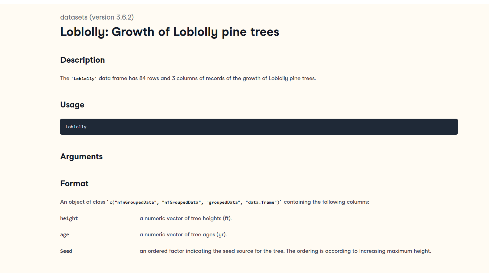
The Loblolly Dataset
The new unit test and example will be based on the Loblolly dataset which is one of the builtin datasets. I chose this data set because it has repeated measurements so it fits the data structure that the BF_for_everyone() function was designed to work with. The dataset is described on rdocumentation.org as follows:
Let's pull a quick Search Labs | AI Overview to get a bit more context.

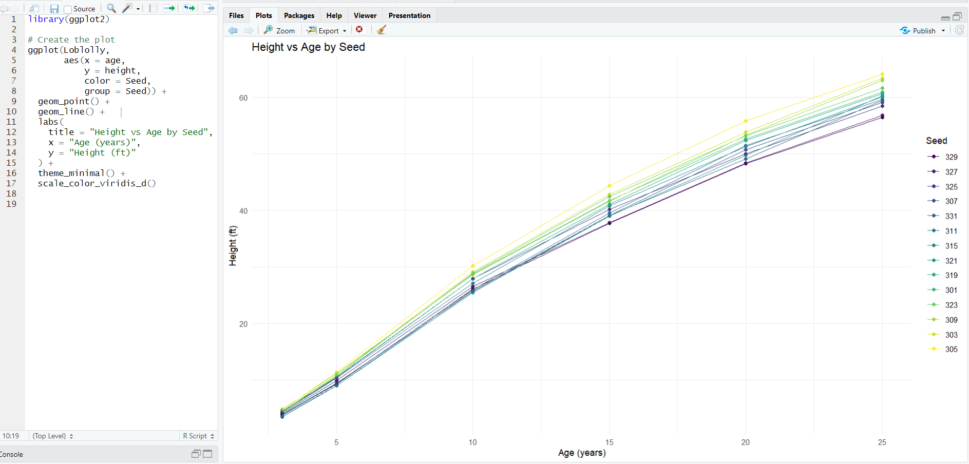
And let's also build a quick ggplot2 visualization of the data:
The new unit test and example for BF_for_everyone() will use the the Loblolly dataset to fit a height ~ age linear model with the hypothesis age > 2.5. You can find this example and unit test on the Mighty Metrika GitHub. In what follows, we will run this statistical model using the BFfe shiny app on mightymetrika.com. We'll structure it as a BFfe tutorial.
BFfe Tutorial
In this tutorial we will use the Loblolly dataset which is built into R to conduct an analysis using the BFfe Shiny application.
Step 1: Open the BFfe App
You can access the app by:
- Going to mightymetrika.com
- Clicking on Tools
- Clicking on BFfe
This will open the Shiny application in your browser. Alternatively, you can open the app through R as follows:
- Open RStudio
- Run install.packages("mmibain") in your console
- Run mmibain::BFfe() in your console
Once you have the app up and running, you should see the following screen:

Step 2: Upload Loblolly Data
Before uploading the Loblolly data to the app we need to make sure we have a copy of the data set in csv format on our hardrive. In R we can accomplish this with the code:
write.csv(Loblolly, file = "Loblolly.csv", row.names = FALSE)
I ran this code on my computer to produce the data set that you can download using the button below.
Now you can upload this data to the BFfe app as follows:
- Click the BROWSE... button
- Navigate to Loblolly.csv on your hard drive
- Select Loblolly.csv
- Click Open
If everything worked, you should see the following screen.
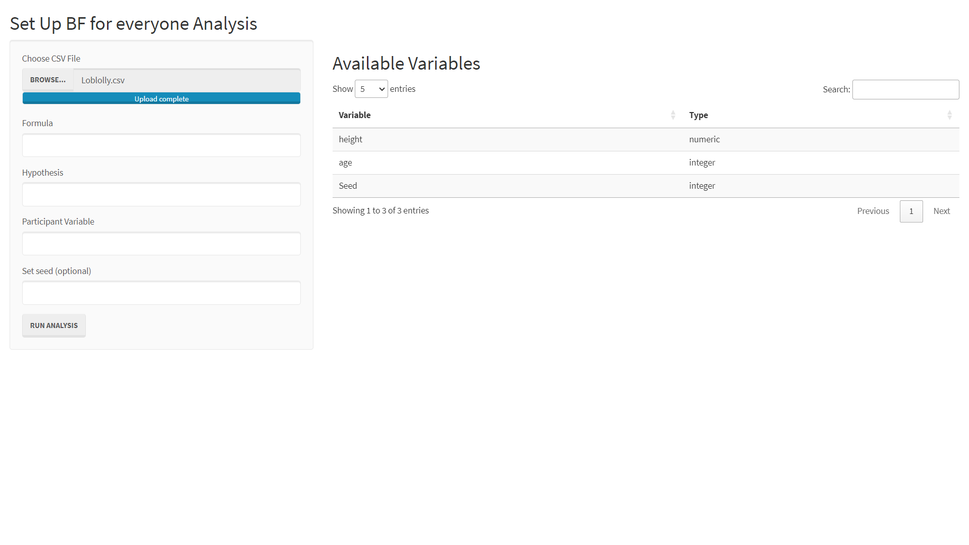
Step 3: Set-up the Run
Now to set-up and the run the analysis we need to:
- Enter the Formula: height ~ age
- Enter the Hypothesis: age > 2.5
- Enter the Participant Variable: Seed
- Click Run Analysis
Our results will not match exactly since we are not using a seed. But after completing these steps, you should see results that look like the following:
Step 4: Interpret Results
For a full introduction to interpreting results from 'bain', I recommend A Tutorial on Testing Hypotheses Using the Bayes Factor.
In our example we are testing the hypothesis H1: age > 2.5 for each seed. Notice that the note in the 'bain' output that states:
"BF.u denotes the Bayes factor of the hypothesis at hand versus the unconstrained hypothesis Hu. BF.c denotes the Bayes factor of the hypothesis at hand versus its complement. PMPa contains the posterior model probabilities of the hypotheses specified. PMPb adds Hu, the unconstrained hypothesis. PMPc adds Hc, the complement of the union of the hypotheses specified."
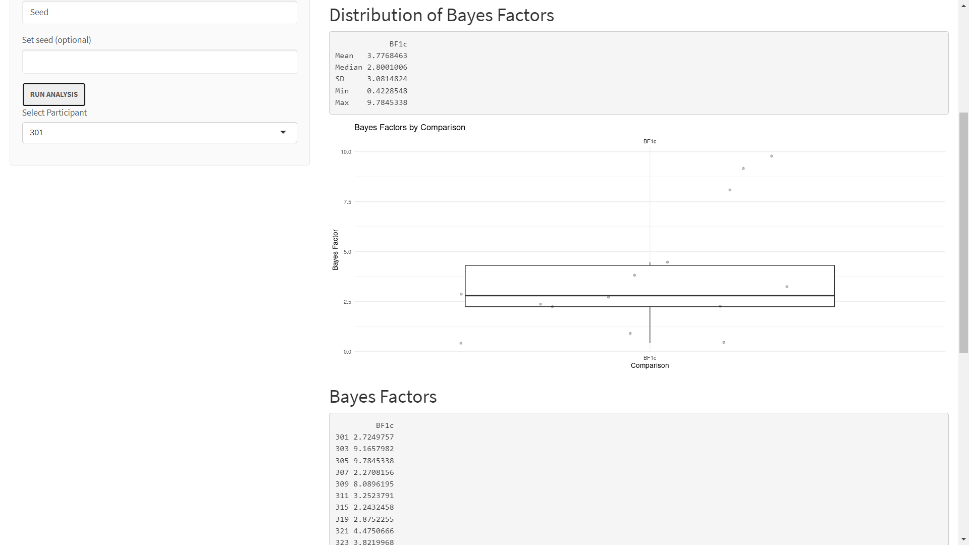
Our main focus in this analysis is BF.c for H1 which is labeled BF1c. In A Tutorial on Testing Hypotheses Using the Bayes Factor BF.c is described as follows:
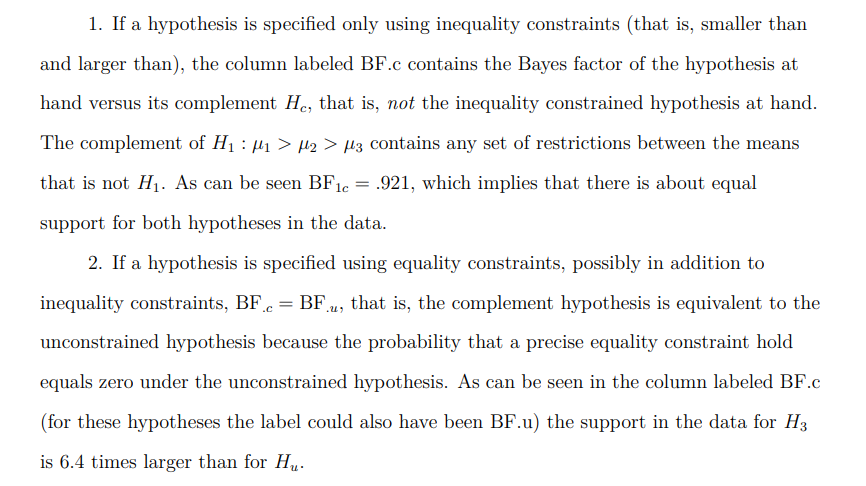
The first section of the results, Distribution of Bayes Factors, just returns descriptive statistics and a boxplot of the BF1c for each seed. This section shows us that the median BF1c is over 2.5.
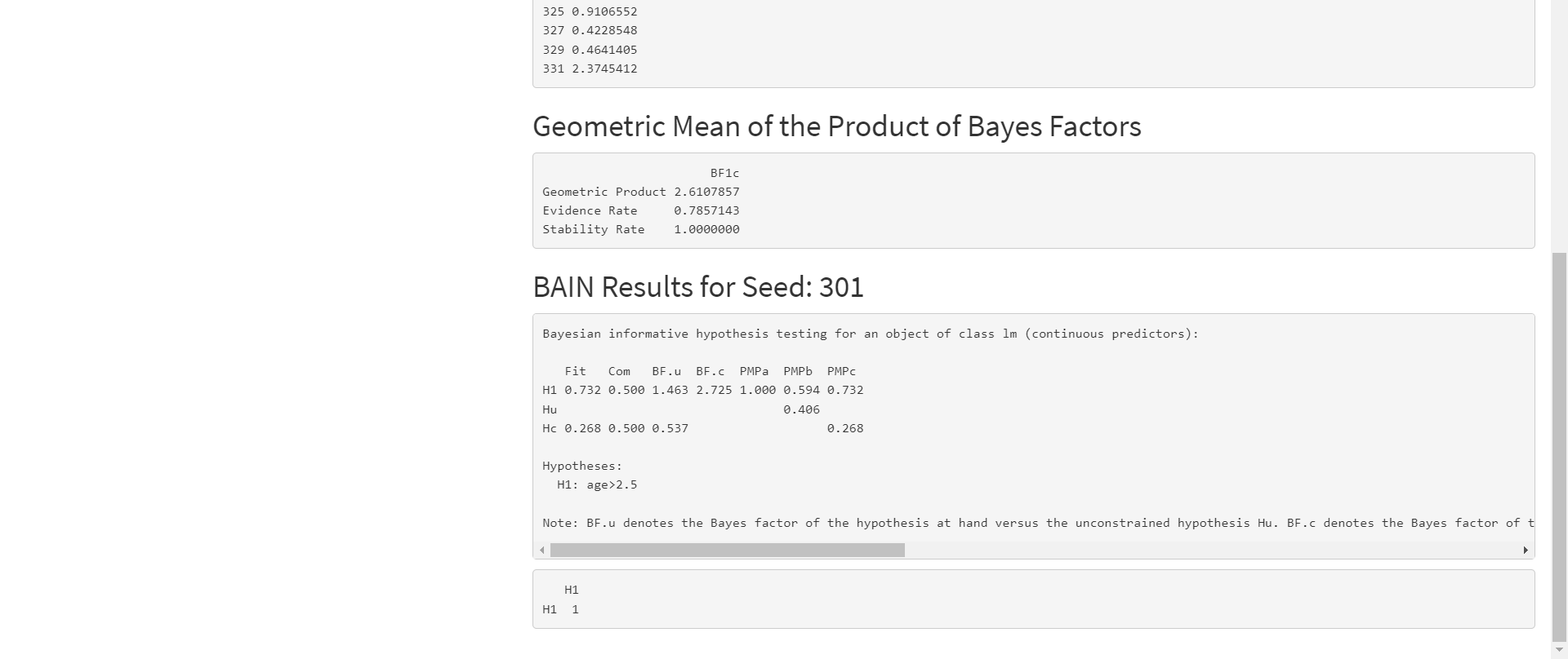
The Geometric Mean of the Product of Bayes Factors presents metrics introduced in the Klassen's paper:
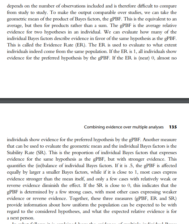
The gPBF in our example suggests that the average seed's evidence is 2.61 times stronger in favor of our hypothesis compared to the complement. The ER of 0.79 suggests that 79% of the seeds have evidence in favor of our hypothesis compared to the complement.
The last section, BAIN Results for Seed: 301, shows the 'bain' output for a particular seed. You can use the Select Participant drop down underneath the Run Analysis button to select a different seed.